Mix Path Selection

[mghazwi]

Mix Path Selection

In this research post, we try to summarize the research and simulations done to better understand the malicious path problem and how much anonymity we can expect when a long-term connection/session is maintained over the Mix protocol. Examples of such sessions are anonymous downloads and hidden services (for some context about the problem, see the research post).

We basically want to understand two things:

1. How bad is this in practical settings? We can theoretical compute this with mathematical formulas and bounds and we can simulate this to get some numbers as well.
2. Can we improve (i.e., decrease) the probability of de-anonymization by changing the path selection strategy? We can design path selection strategy for our use-case and mixnet setting by building on prior work which include: the Tor Guard and Vanguard protocols, the Bow-tie strategy, and the other recent strategies proposed in the NDSS paper.

In here we will focus on session-based mix path selection specifically for anonymous download over the transport layer and we will discuss and explore possible time-based mix path selection strategies for hidden services in a separate post.

We can define a download session as a single or multiple transport layer sessions where a client requests and receives multiple chunks/files that are related, i.e., the chunks are all related to the same file or multiple files but all belong to the same content category/type.

Threat Model & Adversaries

In order to understand how good or bad a certain strategy for selecting a path is, we need to define our threat model. Mixnets in general are designed to provide anonymity and protect against “Global Passive Adversaries” (GPA) which can observe all traffic on the network. To help achieve this, mixnets select a path (of L hops) uniformly at random from the set of online mix nodes. While this minimizes how much the GPA can observe, it doesn’t account for the fact that most network traffic consists of sessions rather than single packets (though the original mix design doesn’t account for this because it was designed for emails, so single packets were expected).

In a session, the two communicating parties will exchange multiple packets and for each one, they will select a path. If we assume a pecentage of the network is controlled by malicious mix nodes (e.g., 10%), then the more packets needed for a session, the more chance that a path containing all malicious nodes is possible. Therefore, if we expect traffic in the mix network to consist of sessions (and we do since we plan anonymous download and possibly hidden services), then we need to consider the malicious mix node adversary in our threat model. We can refer to this adversary as MMN.

With these two adversaries (GPA and MMN), we need to balance how much advantage we give to each:

• selecting paths uniformly at random minimizes the advantage given to GPA and maximizes it to MMN.
• selecting a single path for the whole session (similar to Tor) maximizes advantage for GPA and minimizes it for MMN.

Measuring anonymity

The path selection strategies that we explore in this post will try to balance the advantages given to each of these advarsaries, but first we need some metrics to measure this advantage.

As a starting point, we can use the metric from the NDSS paper with some slight modification. Let’s start with some notation:

• L is the number of mix nodes in a path.
• \mathcal{M} is the set of online mix nodes.
• m=|\mathcal{M}| is the number of online mix nodes.
• \mathcal{A}\subseteq\mathcal{M} is the set of malicious nodes.
• a=|\mathcal{A}| is the number of malicious nodes.
• \beta=a/m is the malicious fraction of the network.
• q is the probability that one sampled path is fully compromised.

For a free-route mixnet that samples L distinct nodes uniformly at random, we can calculate this as:

q = \beta^L.

Given these notations, we can now define the metrics as follows:

1. DLM: the de-anonymization likelihood metric estimates the probablity of picking a fully malicious path (a path of L nodes that are all malicious). Depending on the use-case, DLM can be calculated differently. For us we consider the three main formulas:

• packet-based DLM (P-DLM): the probability of selecting a malicious path with L hops from the set of online mix nodes \mathcal{M} where we expect \beta percentage of it to be malicious:

  \texttt{P-DLM}=q = \beta^L

  For example, if the adversary controls 10\% of the nodes and paths contain three independently selected hops, then

  \texttt{P-DLM}=0.1^3=0.001

  Thus, approximately one out of every 1000 independently sampled paths is expected to be fully compromised.

• session-based DLM (S-DLM): is the probability that at least one packet in a session uses a fully compromised path.
  Consider a session containing N packets. If the path used by each packet is selected independently and every path has compromise probability q, the probability that none of the packets uses a fully compromised path is:

  (1-q)^N

  The probability that at least one packet uses a fully compromised path is therefore:

  \texttt{S-DLM}(N) = 1-(1-q)^N = 1-\left(1-\beta^L\right)^N

  e.g., for a 2 KB packet payload and one return path per packet, a 4 MB transfer needs approx N=4096 paths (ignoring acks and redundancy, etc). With \beta=0.1, L=3:

  \texttt{S-DLM}(4096)\approx 98\%.

  Note: this formula assumes that packet paths are independent. We will need to adjust it later for strategies that reuse paths, fixes hops, or selects hops from a set with differnt \beta values.

• time-based DLM (T-DLM): extends S-DLM to a long-lived hidden service exposed to repeated requests from malicious clients. To get an approximation for T-DLM, we can restrict the lifetime of the hidden service to T and work out a formula for computing T-DLM. We will define and discuss this further in a separate post.

2. CAM: the “correlation advantage metric” measures the predictability of the routes during client-service sessions from the perspective of a GPA. Traffic concentrated on a small number of paths is more predictable than traffic distributed uniformly across many paths. We will skip computing this for the time being and will come back to it later on, possibly in a separate research post since measuring this also depends on the dummy traffic strategy used in mix.

The free-route simulator (freeroutesim)

Aside from the computation using formulas, we can simulate the path selection using a simulator. We have a (work-in-progress) simulator for free-route mix which we will use. It builds on ideas from previous works that use stratified mixnet. The free-route mix simulator contains three main components:

• the topology genrator: takes a mixnet params and assumptions and generates a mixnetwork (set of mix nodes) for the required number of epochs (time-periods).
• the user model: describes the communication behaviour being simulated and defines what it means for a path to be compromised.
• the path sampler: implements the path-selection strategy being evaluated.

The implementation for this simulator can be found here: GitHub - logos-storage/hs-mix-sim: Hidden Services over Mix simulations · GitHub
We describe these in the following sections.

Free-route Mix Setting

Previous papers (1, 2) consider a statified mix. That means the Mix is divided into L layers, where L is usually the number of hops that mix messages will go through (L is usually 3). Active Mix nodes are then assigned to each of these layers and each message is routed through one mix node from each layer. This is different from a free-route mixnet, where the sender can choose an arbitrary sequence of mix nodes:

1. Sender discovers a set of active/online mix nodes from the mix pool.
2. Sample L nodes from the active mix nodes and assign each to a hop in the path.
3. use the path to send a message.

Topology Generator

The topology generator creates a set of mix nodes with their associated properties (e.g. malicious, weights, and additional properties) representing the mix network for each epoch. We define epochs as time periods in which these mix nodes and their properties are valid. The generator determines which nodes exist, which nodes are online, the properties associated with each node, and models changes in the network, such as nodes joining, leaving, going offline, or returning online.

The generator takes the following main params:

Parameter	Default
Mix nodes (m)	1,000
Malicious node-fraction (\beta)	10%
Malicious bandwidth-fraction target (\rho)	10%
Churn probability per epoch (\psi)	3%
Epoch duration (\epsilon)	3,600 sec

Based on these parameters, the topology generator would output a number of topologies depending on the configration, where each topology represent a time snapshot of the network that shows online mix nodes and their properties during that snapshot/epoch. It can also output a single topology which is usefull for session-based simulations where a session (e.g. download session) usually doesn’t span multiple epoch (we consider epochs to be somewhat long e.g. 1-2 hours and so a download session is assumed to no last more than that hopefully).

the models

We will focus on the anonymous download over the transport layer in our evaluation of the path selection strategies. In the following, we define a model that simulates this.

Anonymous download

We will assume, as mentioned earlier, that each user performs a single download in a single topology snapshot. This is mainly because users can only be correlated within a single session, and different sessions cannot be linked given our definition of a session.

To model the anonymous download over the transport layer as accurately as possible, we need to model the chunking, erasure coding, SURB supply, and transport/control overhead traffic from the transport layer protocol.

The model needs to define the user behaviour: how many packets are sent and when?
We assume all packets in a session are sent in a single epoch and so we are not considering time here. We can approximate the number of packets based on a few parameters:

• F be the download file(s) size in bytes
• P(L) be the usable Sphinx payload (\delta) size for a path of L hops
• H_T be the transport-layer overhead added to each data chunk. This is a constant value.
• R(L)=P(L)-H_T be the amount of file data that fits in one transport chunk.
• r = \frac{n}{k} where 1 \leq r \leq 2 be the erasure-coding redundancy ratio
• S_{\mathrm{SURB}}(L) be the size of one L-hop SURB.
• N_\texttt{session} be the number of sphinx packets needed to complete the session, i.e. the number of paths selected by the downloader for both forward and backward (SURBs) packets.

The number of chunks needed for the file is basically a function of F and L:

K(F,L) = \left\lceil \frac{F}{R(L)} \right\rceil.

After adding erasure-coding redundancy, the number of provider-to-downloader data packets is

N_D(F,L,r) = \left\lceil rK(F,L) \right\rceil

Since the downloader is anonymous, each return packet from the provider requires one SURB. Therefore, approximately N_{\mathrm{SURB}}=N_D SURBs must be supplied to the provider.

The number of SURBs that fit inside one forward transport packet is:

C_{\mathrm{SURB}}(L) = \left\lfloor \frac{P(L)-H_T} {S_{\mathrm{SURB}}(L)} \right\rfloor.

The number of downloader-to-provider packets needed to supply these SURBs is then:

N_F = \left\lceil \frac{N_D} {C_{\mathrm{SURB}}(L)} \right\rceil.

We can additionally assume a $5$ overhead for transport-control traffic such as requests, acknowledgements, session control, and SURB-management messages that are not already captured above. The total number of Mix packets in the session is therefore approximated as:

N_{\texttt{session}} = \left\lceil 1.05\left(N_D+N_F\right) \right\rceil

We can then substitute the previous terms and compute the number of packets needed for the simulated session as a function that depends on:

• the download file size
• number of hops in the mix path
• the erasure coding redundancy ratio/rate

N_{\texttt{session}}(F,L,r) = \left\lceil1.05 \left( \left\lceil r \left\lceil \frac{F}{R(L)} \right\rceil \right\rceil + \left\lceil \frac{ \left\lceil r \left\lceil F/R(L) \right\rceil \right\rceil}{C_{\mathrm{SURB}}(L)} \right\rceil \right) \right\rceil

We assume the erasure-coding redundancy is sufficient and so we don’t account for retransmissions. If EC reconstruction fails, the session is considered failed and a new session would be required.

The computed approximate number of packets N_{\texttt{session}} will then be used in the simulation to evaluate the different path selection strategies.

For an anonymous download, we define the session as compromised if at least one fully malicious path is selected at any point during the session.

Path samplers/selectors

Uniform random (UR)

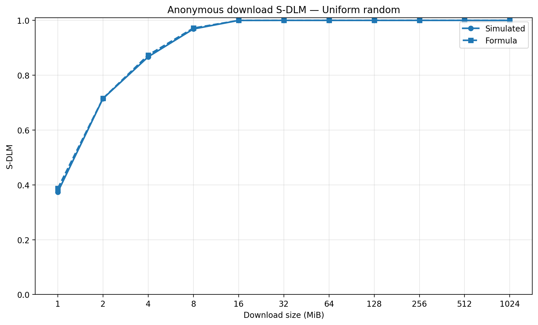
Every hop is sampled uniformly from active nodes without repeating a node within the path. A fresh path is sampled for every message. This is the currently used path selection strategy used in the mix protocol and will serve as base-line for other strategies. We can use the same \texttt{S-DLM} formula for this

\texttt{S-DLM}_{\mathrm{UR}}(N) \approx 1-\left(1-\beta^L\right)^N.

Note we are ignoring the small without-replacement difference here.

Bandwidth random (BR)

Every hop is sampled in proportion to node bandwidth/reputation weight. Duplicate nodes are rejected, so the resulting path is a bandwidth-weighted sample without replacement.

Since we are sampling based on bandwidth/reputation weight, then we need to replaces the malicious node fraction \beta with the malicious weight fraction \rho, which equals to the percentage of weight controlled by malicious nodes. Then we can use the same formula as above:

\texttt{S-DLM}_{\mathrm{BR}}(N) \approx 1-\left(1-\rho^L\right)^N,

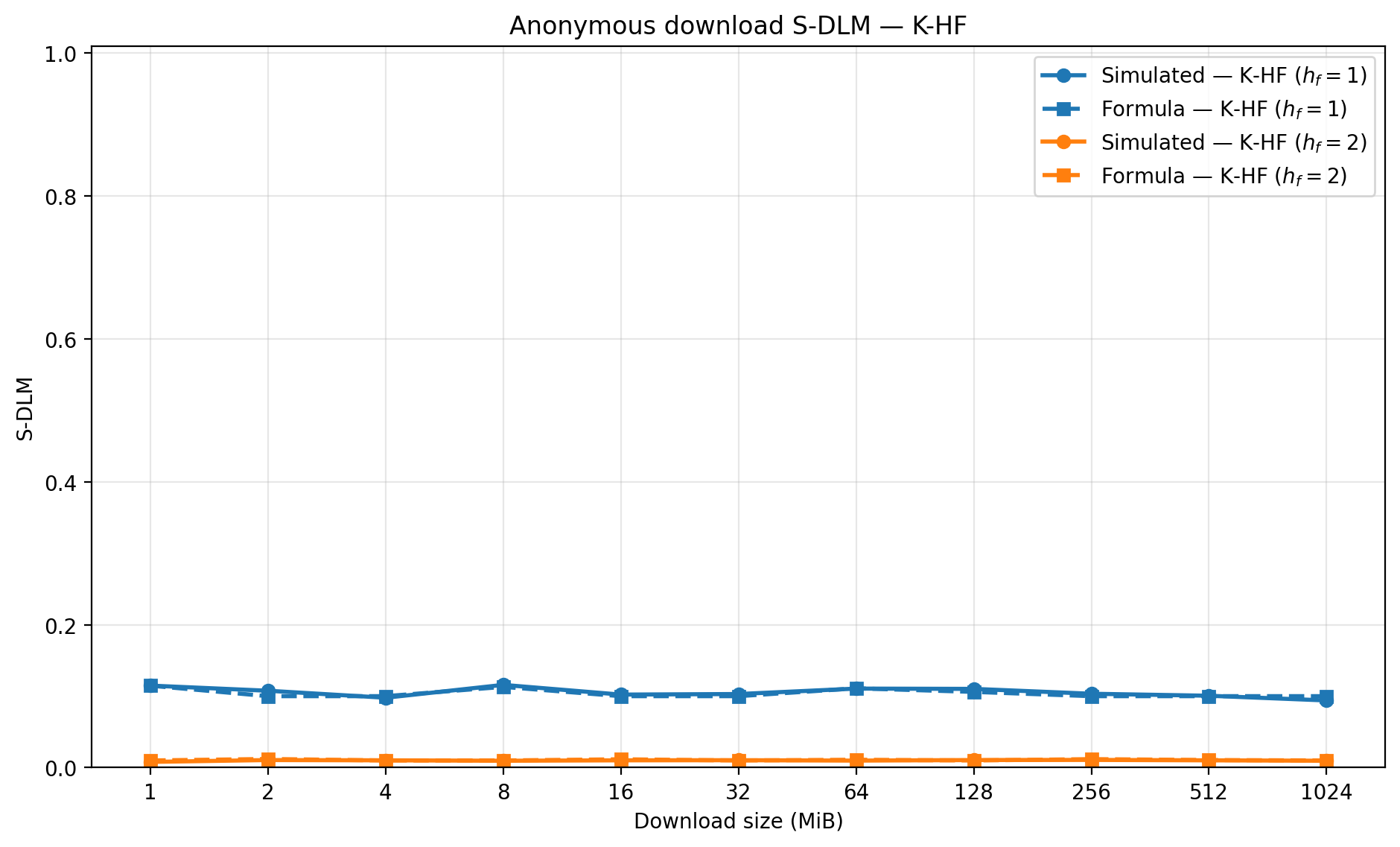
K-HF Strategy

The idea is that K-HF splits the L hops path into two parts:

• h_f fixed positions. At each position we maintain a single node that stays unchanged for the whole session.
• L-h_f positions with nodes that are randomly resampled for every packet.

Given these conditions, for a malicious path to be chosen, two things must happen:

1. All fixed nodes are malicious. Since each fixed node has probablity \beta of being malicious, then this happens with probability \beta^{h_f}. If a single fixed position contains all honest nodes, then the session will never have a malicious path.

2. The remaining L-h_f nodes that are not fixed are all also malicious. The probability that all L-h_f randomly chosen nodes are malicious is \beta^{L-h_f}, therefore, the probability that at least one of the paths in the non-fixed positions in a session ( with N paths selected) contain all malicious nodes is 1-\left(1-\beta^{L-h_f}\right)^N which is basically the same as \texttt{S-DLM} above since we are randomly selecting nodes for these positions.

Multiplying the two required events gives us the formula for this path selection strategy:

\texttt{S-DLM}_{\mathrm{K\text{-}HF}}(N) \approx \beta^{h_f} \cdot \left(1-\left(1-\beta^{L-h_f}\right)^N\right)

we can see here that for large N:

\left(1-\beta^{L-h_f}\right)^N \to 0

so:

1-\left(1-\beta^{L-h_f}\right)^N \to 1

meaning that what we compute is eventually just \beta^{h_f} which is the probability that our initial pick for these fixed hops is fully malicious. For example, fixing a single hop in the path and assuming large number of packets/path sampled (N), then the probability or de-anonymization during that session comes down to whether or not the fixed hop is malicious, since in mix as long as a single hop in the path honest, anonymity is preserved. Therefore, if we assume malicious control is \beta = 0.1, then there is 10% chance of deanonymization with the single fixed hop. we can lower that with fixing more hops, e.g., two fixed hops and 0.1^2 = 0.01 then 1% chance of deanonymization.

K/W Strategy

In this strategy, we create persistent sets containing K uniformly selected nodes from the online/live mix nodes W for each hop position. i.e., we will have L sets, each of size K, so S = (s_1,s_2,\ldots,s_L,) where |s_j|=K. Note that here W=m because we are considering a free-route mix and so we sample from all online mix nodes and note from layers as in stratified mix.

For a fully malicious path to be possible, we need the following two conditions to happen:

1. every set in S must contain at least one malicious node. If a single set doesn’t contain a malicious node, then malicious paths will never happen.
2. One of the session’s N packets actually selects malicious nodes from all pools simultaneously.

The first condition requires modeling the malicious fraction inside each K-node pool using the hypergeometric distribution. This gives us the probability of selecting a malicious node from the pool in s_j:

\beta_j \sim \texttt{Hypergeometric}(W,\beta W,K)

where \beta_j is the malicious fraction in set s_j, W is the number of nodes from which the set is sampled, \beta W is the number of malicious nodes, and K is the set size. Again in our setting, W=m.

We use the hypergeometric distribution because each fixed set contains K distinct nodes sampled without replacement from the mix pool with a known malicious fraction \beta. The hypergeometric distribution therefore models how many malicious nodes end up in each set.

Now, to get the probability that one packet selects a fully malicious path is basically:

q = \prod_{j=1}^{L}\beta_j

For a session of N packets, the probability that at least one packet is compromised (fully malicious) is just plugging q into \texttt{P-DLM}:

1-\left(1-q\right)^N = 1- \left( 1- \prod_{j=1}^{L}\beta_j \right)^N

Because the values \beta_j depend on the randomly generated sets, we need to compute the expected value over their possible combinations. Therefore, the resulting formula for the probability as used in the paper is:

1-\mathbb{E} \left[ \left(1-\prod_{j=1}^{L}\beta_j\right)^N \right]

However, as suggested by the paper, we can use a simpler upper bound approximation:

There are at most K^L distinct paths that can be formed from the fixed sets. A session with N packets can therefore use at most \min(N,K^L) distinct paths.

Approximating each distinct path as having compromise probability \beta^L (similar to a randomly selected path, but in reality it should be less because paths selected from fixed sets are not truly independent), we get:

\texttt{S-DLM}_{\mathrm{K/W}}(N) \lesssim 1- \left(1-\beta^L\right)^{\min(N,K^L)}

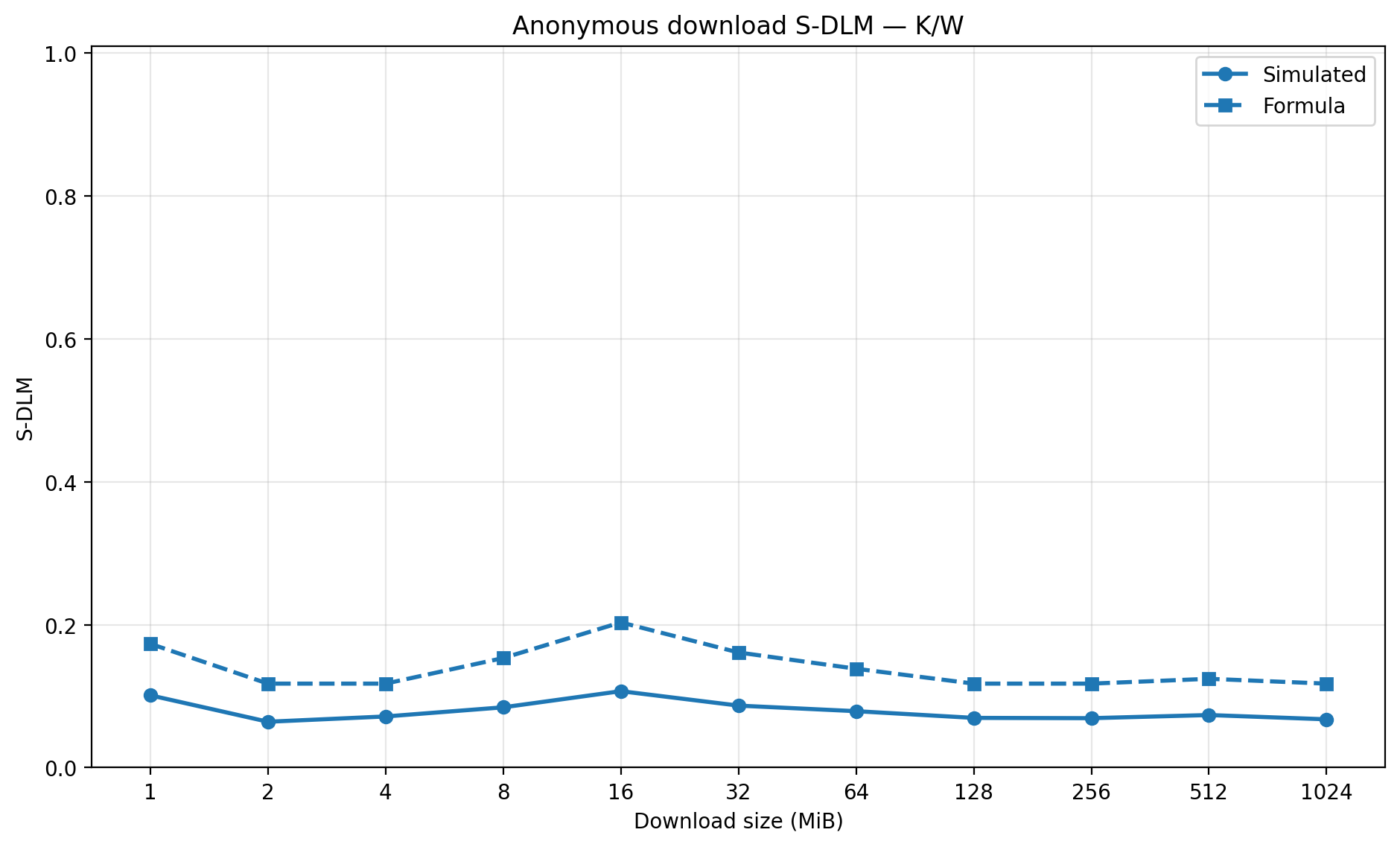
Observe that this is basically the same as the formula for \texttt{S_DLM} and only improves it when K^L < N. We will use this approximation formula for our evaluation of this path selection strategy, but simulation numbers are expected to be less than this upper bound.

Alpha-Sticky Selection (alpha-SS) Strategy

Alpha-SS strategy maintains a set S_\alpha which contains the paths used to send packets through mix.

The set S_\alpha starts empty and so you sample the first path uniformly and add it. For every later packet it:

• Sample a path from S_\alpha with probability \alpha or
• samples a new, previously unused path from the online mix nodes with probability 1-\alpha. This path is used and added to S_\alpha.

Let q=\beta^L be the probability that a uniformly selected path is fully malicious, then the paper suggests this formula:

\texttt{S-DLM}_{\alpha\text{-SS}}(N) \approx 1-(1-q) \prod_{i=2}^{N} \left[ \alpha+ (1-\alpha) \left( 1- \frac{m^L q} {m^L-1-(1-\alpha)(i-2)} \right) \right]

This looks quite complex, but let’s try to unpack it:

• when you have no path in S_\alpha and you pick one randomly there is q=\beta^L chance of that path being malicious. So it will be safe with probability 1-q.
• we re-use existing paths with probability \alpha
• new path are selected with probability 1- \alpha, and the there is let’s called it q' chance that these paths are malicious. The paper computes this q' as:
  q' = \frac{m^L q}{m^L-1-(1-\alpha)(i-2)}

what this fraction basically says is that we are dividing the number of malicious paths (m^L q) by the total number of paths after removing the ones we selected (m^L-1-(1-\alpha)(i-2)). What we are removing is: 1 for the first path, (1-\alpha)(i-2) the appoximate number of path we selected previously which depends on \alpha.

m^L - \underbrace{1}_{\text{first selected path}} - \underbrace{(1-\alpha)(i-2)}_{\substack{\text{expected number of additional}\\\text{new paths selected earlier}}}

• Now if we put all the previous ones together, we get the paper’s suggested formula.

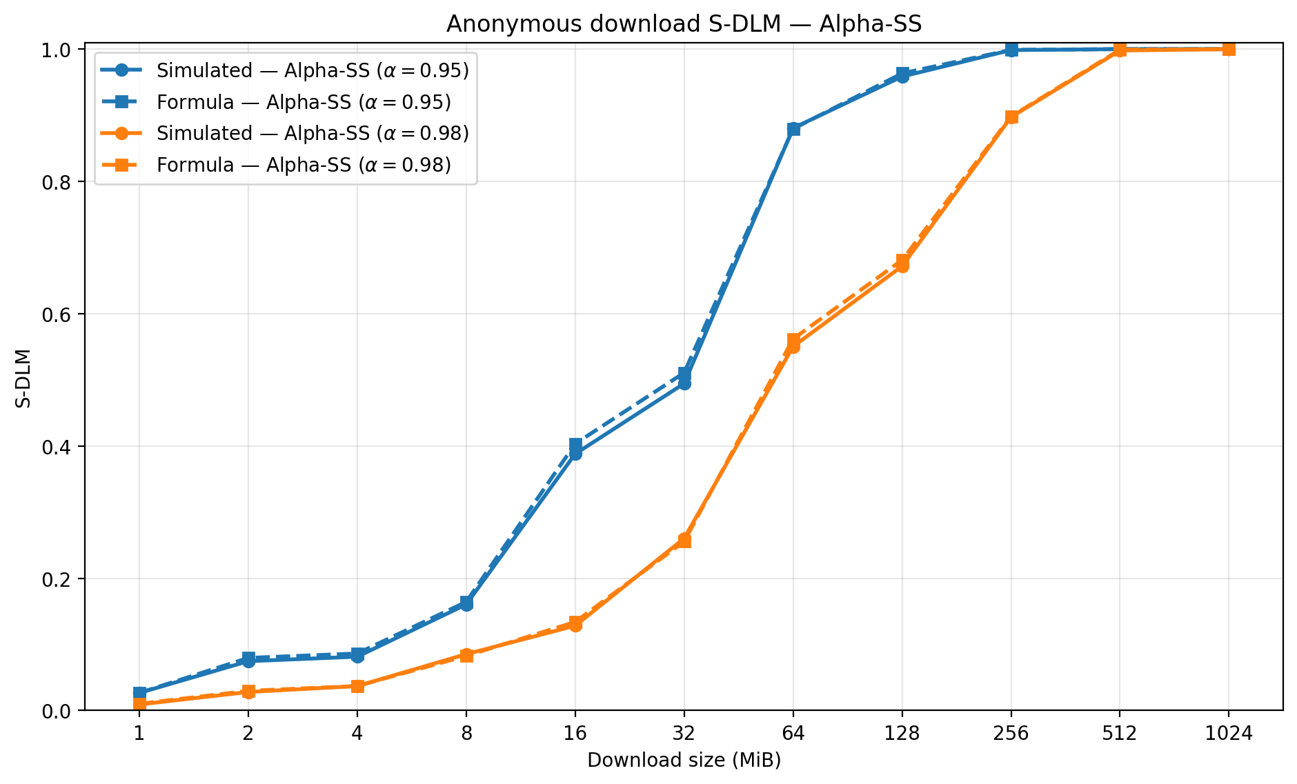
However, if we simplify and assume each path is sampled independently, i.e., q' = q (meaning we are ignoring the fact that the path pool we are selecting from gets smaller and smaller as we sample more paths), then we have:

\alpha+(1-\alpha)(1-q) = 1-(1-\alpha)q

This simplifies the formula to:

\texttt{S-DLM}_{\alpha\text{-SS}}(N) \approx 1-(1-q)\left(1-(1-\alpha)q\right)^{N-1}

The Bow-Tie, Guard, Vanguards Strategy

This approach is from the research paper: Stopping Silent Sneaks: Defending against Malicious Mixes with Topological Engineering. The paper also provides a tool to simulate and get some estimations. The approach is similar to the Tor Guard protocol but applied to a stratified mixnet. Similar to Tor, Bow-Tie starts by generating a list of stable & high-bandwidth relay/mix nodes which serve as a stable guard layer (not necessarily honest, they can still be malicious), and clients can then select from this layer. Bow-tie assumes a configuration server (or a consensus) that assigns the guard nodes similar to Tor directory authorities. The guard layer is fixed to either the first or second hop (in our implementation it is the second hop). This layer is updated at each epoch. We can summarize the client selection logic as follows:

• client samples a list of guards (default = 5 nodes). Sampling can be random, weighted by bandwidth, or from consensus-tagged active guards.
• client starts by picking the first in the set i.e., guards[0] as the selected guard
• at each epoch, it loops through the set of guards and picks the first online one, i.e., if the selected one guards[0] is online it will keep using it until it’s offline. When it is offline it will move to the next available one e.g., guards[1]. Later when old selected one goes back online, it will be the one selected again.
• the list is extended by one only if no existing candidate is online.
• All non-guard positions are freshly sampled (optionally by bandwidth).

Note that the bow-tie approach works best when considering time e.g., time-based DLM because it considers bandwidth and stability which would mean less chance of guard nodes going offline and needing to pick new ones. However, when consider download sessions, time doesn’t play much of a factor, and so this strategy (and the guard/vanguard) reduce to basically fixed hops i.e., the K-HF strategy and formula above.

Evaluation of path selection

Method

Each run produce both computed values based on the S-DLM formula for the chosen strategy, and the simulated value as well. We evaluated the following strategies:

• uniform random
• K-HF
• K/W
• alpha-ss

Each simulated run generates a fresh topology. Therefore, the realized malicious fraction can differ between runs. The curve uses the beta calculated from that run’s actual topology, so the computed value uses the same beta as the simulated one.

Configuration

Parameter	Value
simulated runs	5,000
Path hops L	3
Total Sphinx packet size	4608 bytes
K-HF fixed-hop variants	h_f=1, h_f=2
K/W sets	K=5
Alpha-SS	\alpha=0.95, \alpha=0.98
File sizes	2^0 - 2^{10} MiB

Uniform random

K-HF

K/W

Alpha-SS

Results Summary

As can be seen above, K-HF seem to produce the least value for S-DLM followed by K/W. It is therefore best to probably follow such an approach when selecting a path for anonymous download. This is also the approach that mostly resembles the guard protocol which might not be so surprising why Tor is using it. The simplest approach seem to be the best approach in this case which is to just fix few hops. The fixed hops would ideally be selected from somewhat trusted nodes rather than random but that still doesn’t change the fact that there is still a pecentage of these nodes that could be malicious or possibly turn into malicious at a later stage. However, the percentage of malicious control in a trusted pool of nodes is expected (hopefully) to be lower than in all public nodes. This doesn’t change the formula, only lowers the expected malicious control \beta.

In general, it might be best to consider a hybrid approach that combines both K-HF and K/W considering that mix node stability/churn might be a factor in a realistic download setting. A hybrid approach would be to select a k-size set for each fixed hop, stick to the first hop and only change to the next/random one from the set when that node is not online. A detailed description of this is currently being written in the mix path selection spec. Such an approach would also work in the hidden service setting. A more detailed discussion on this will be posted in a separate research post.